Introduction of Batch Effect Correction
The batch effect correction analysis module performs an automatic or specific correction on the peak data table generated by peak picking step. Multiple correction methods have been embedded inside. They include combat, WaveICA, EigenMS, QC_RLSC, ANCOVA, RUV_random, RUV_2, RUVseq series (RUV_s, RUV_r and RUV_g), NOMIS, CCMN. The detailed limitation and mathmatic mechanism of different methods have been illustrated in our manuscript. Here, 4 cases is provided to show users a step to step workflow for both batch effect and signal drift correction.
Data preparation
The peak table generated by FormatPeakList function needs to be manually prepared by hand to supplements the corresponding information below.
-
1st column The samples name;
-
2nd column Sample groups/classes information, if there are any QC samples, please mark them as QC;
-
3th column Batch information, please provide consistent characters within the same batch;
-
4th column order information, please provide injection order information of the whole samples;
-
other column Features’ intensity should be provided. If any internal standards, please mark the feature with “IS”.
NOTE: Please provide as more information as possible. If some information omitted, please leave the columns empty.
Here is an example table.
| S1 |
UC |
B1 |
1 |
3420.067 |
3595.400 |
3403.082 |
3422.175 |
3616.583 |
| S2 |
UC |
B1 |
2 |
3332.439 |
3522.818 |
3666.475 |
3454.279 |
3419.392 |
| S3 |
UC |
B1 |
3 |
3384.851 |
3705.339 |
3620.226 |
3554.620 |
3438.895 |
| S4 |
UC |
B1 |
4 |
3593.815 |
3574.260 |
3620.767 |
3561.398 |
3365.505 |
| QC1 |
QC |
B1 |
5 |
3396.274 |
3407.036 |
3529.572 |
3516.900 |
3383.464 |
| QC2 |
QC |
B1 |
6 |
3400.617 |
3497.153 |
3626.562 |
3573.033 |
3505.492 |
| S5 |
UC |
B1 |
7 |
3507.520 |
3353.179 |
3548.650 |
3428.837 |
3678.415 |
| S6 |
UC |
B1 |
8 |
3454.916 |
3569.033 |
3669.644 |
3312.210 |
3394.256 |
| S7 |
CD |
B1 |
9 |
3628.472 |
3484.903 |
3526.993 |
3655.381 |
3476.667 |
| S8 |
CD |
B2 |
10 |
3639.546 |
3481.560 |
3502.178 |
3724.512 |
3535.429 |
| QC3 |
QC |
B2 |
11 |
3585.290 |
3602.893 |
3546.777 |
3396.528 |
3519.941 |
| QC4 |
QC |
B2 |
12 |
3596.886 |
3474.214 |
3666.306 |
3646.229 |
3473.409 |
| S9 |
UC |
B2 |
13 |
3604.571 |
3594.637 |
3347.312 |
3334.772 |
3419.270 |
| S10 |
CD |
B2 |
14 |
3320.749 |
3421.437 |
3542.846 |
3432.795 |
3431.518 |
This Benchmark data is a large batch data with over 600 samples. The data file size is over 70 MB. This part is designed for repeating our published results. Running of this part may take over 30min to finish. You are strongly recommonded to use your own data instead of this large file to avoid the consuming of patience.
Data Downloading and Preparation
# Use Google API for data downloading peak feature data generated by FormatPeakList here.
# Please "install.packages('googledrive')" and "install.packages('httpuv')"first.
library(googledrive);
temp <- tempfile(fileext = ".csv")
# Please authorize your google account to access the data
dl1 <- drive_download(
  as_id("1wEh2P81J_xFWJs5y4mq98-FsjxJ5wmBO"), path = temp, overwrite = TRUE)
# Use Google API for data downloading meta data here.
# Please "install.packages('googledrive')" and "install.packages('httpuv')"first.
library(googledrive);
temp <- tempfile(fileext = ".csv")
# Please authorize your google account to access the data
dl2 <- drive_download(
  as_id("1KaBnSNRrirVPvpRxIubGCqpjX8asNeVA"), path = temp, overwrite = TRUE)
## File downloaded:
##   * metaboanalyst_input.csv
## Saved locally as:
##   * /tmp/RtmpIBzO2x/file11c64ad429b2.csv
## File downloaded:
##   * meta_data.csv
## Saved locally as:
##   * /tmp/Rtmp3haVCa/file90a5282e7b0.csv
# Data preparation - read data in & transpose.
# This is a reference example for user to prepare their data.
# Please prepare your data table according to your data format.
MetaboAna_Data <- t(read.csv(dl1$local_path,header = T));
colnames(MetaboAna_Data) <- MetaboAna_Data[1,];
MetaboAna_Data <- MetaboAna_Data[-1,];
MetaboAna_Data <- MetaboAna_Data[order(rownames(MetaboAna_Data)),];

meta_data <- read.csv(dl2$local_path);
meta_data <- meta_data[order(meta_data[,1]),c(1,2,4)];

Prepared_Data <- cbind(meta_data,MetaboAna_Data)[,-4];
write.csv(Prepared_Data,file = "IBD_BC_correction.csv",row.names = F)
datapath <- paste0(getwd(),"/IBD_BC_correction.csv")
Library Package
# Load the MetaboAnalystR package
library("MetaboAnalystR")
Data Filtering and Normalization
mSet<-InitDataObjects("pktable", "stat", FALSE)
## Starting Rserve:
##  /usr/lib/R/bin/R CMD /home/qiang/R/x86_64-pc-linux-gnu-library/4.0/Rserve/libs//Rserve --no-save
##
##
## R version 4.0.0 (2020-04-24) -- "Arbor Day"
## Copyright (C) 2020 The R Foundation for Statistical Computing
## Platform: x86_64-pc-linux-gnu (64-bit)
##
## R is free software and comes with ABSOLUTELY NO WARRANTY.
## You are welcome to redistribute it under certain conditions. Type 'license()' or 'licence()' for distribution details.
##
##   Natural language support but running in an English locale
##
## R is a collaborative project with many contributors.
## Type 'contributors()' for more information and
## 'citation()' on how to cite R or R packages in publications.
##
## Type 'demo()' for some demos, 'help()' for on-line help, or
## 'help.start()' for an HTML browser interface to help.
## Type 'q()' to quit R.
##
## Rserv started in daemon mode.
## [1]  "MetaboAnalyst R objects initialized ..."
mSet<-Read.TextData(mSet, dl1$local_path, "col", "disc")
mSet<-SanityCheckData(mSet)
mSet<-ReplaceMin(mSet);
mSet<-FilterVariable(mSet, "iqr", "F", 25)
mSet<-PreparePrenormData(mSet)
mSet<-Normalization(mSet, "MedianNorm", "LogNorm", "NULL", ratio=FALSE, ratioNum=20)
## [1] "Successfully passed sanity check!"
##  [2] "Samples are not paired."
##  [3] "4 groups were detected in samples."
##  [4] "Only English letters, numbers, underscore, hyphen and forward slash (/) are allowed."
##  [5] "<font color="orange">Other special characters or punctuations (if any) will be stripped off.</font>"
##  [6] "All data values are numeric."
##  [7] "A total of 744120 (14.4%) missing values were detected."
##  [8] "<u>By default, these values will be replaced by a small value.</u>"
##  [9] "Click <b>Skip</b> button if you accept the default practice"
## [10] "Or click <b>Missing value imputation</b> to use other methods"
## [1] " Further feature filtering based on Interquantile Range Reduced to 5000 features based on Interquantile Range"
## [1] " Further feature filtering based on Interquantile Range Reduced to 5000 features based on Interquantile Range"
### Data Orgnization
normalized_set <- mSet[["dataSet"]][["norm"]]
ordered_normalized_set <- normalized_set[order(row.names(normalized_set)), ]
### import metadata
meta_data <- read.csv(dl2$local_path)
new_normalized_set <- cbind(meta_data[,2:4], ordered_normalized_set);
write.csv(new_normalized_set,file = "new_normalized_set.csv")
#perform PCA
mSet <- PCA.Anal(mSet)
mSet <- PlotPCAPairSummary(mSet, "pca_pair_0_", "png", 72, width=NA, 5)
mSet <- PlotPCAScree(mSet, "pca_scree_0_", "png", 72, width=NA, 5)
mSet <- PlotPCA2DScore(mSet, "pca_score2d_0_", "png", 72, width=NA,style = 2, 1,2,0.95,0,0)
rm(mSet)

Initializing mSet Object
mSet <- InitDataObjects("pktable", "utils", FALSE)
## [1] "MetaboAnalyst R objects initialized ..."
Data Reading
## we set samples in "row" according to the table format. If your samples are in column, set it as "col".
mSet <- Read.BatchDataTB(mSet, "new_normalized_set.csv", "row")
Automatic Correction
mSet <- PerformBatchCorrection(mSet)
getwd()
## [1] "Correcting using the Automatically method !"
## [1] "Correcting with Combat..."
## [1] "Correcting with WaveICA..."
## [1] "Correcting with EigenMS..."
## [1] "Correcting with QC-RLSC..."
## Cluster size 2216 broken into 551 1665
## Done cluster 551
## Cluster size 1665 broken into 1025 640
## Done cluster 1025
## Done cluster 640
## Done cluster 1665
## [1] "Correcting with ANCOVA..."
## [1] "Best results generated by  EigenMS  !"
# Show the distances between batches
mSet$dataSet$interbatch_dis
##         table  combat_edata WaveICA_edata  EigenMS_edata  QC_RLSC_edata  ANCOVA_edata
##      38.49935      39.42686      38.32145      24.18179      36.58138     38.38796


Data visualization - PCA plotting with groups
## remove the batch column in the corrected result
data_corrected <- read.csv("/home/xialab/Documents/MetaboAnalyst_batch_data.csv")
data_corrected_new <- data_corrected[,-3]
write.csv(data_corrected_new,file = "MetaboAnalyst_batch_data_stats.csv",row.names =  F)
mSet <- InitDataObjects("pktable", "stat", FALSE)
mSet <- Read.TextData(mSet, "MetaboAnalyst_batch_data_stats.csv", "row", "disc")
mSet <- SanityCheckData(mSet)
mSet <- ReplaceMin(mSet);
mSet <- FilterVariable(mSet, "iqr", "F", 25)
mSet <- PreparePrenormData(mSet)
mSet <- Normalization(mSet, "NULL", "NULL", "NULL", ratio=FALSE, ratioNum=20) # No need to normalize again
mSet <- PCA.Anal(mSet)
mSet <- PlotPCAPairSummary(mSet, "pca_pair_0_", "png", 72, width=NA, 5)
mSet <- PlotPCAScree(mSet, "pca_scree_0_", "png", 72, width=NA, 5)
mSet <- PlotPCA2DScore(mSet, "pca_score2d_0_", "png", 72, width=NA, style = 2, 1,2,0.95,0,0)

In addition of the batch effect, signal drift is also an important issue faced by metabolomics study. QC-RLSC can be used to correct both batch effect and signal drift (PMID: 30253838). Here, we showcase an example for user to correct the signal drift with an simulated datatable.
There is one point noted: As for batch effect correction in case 1 and case 2, only batch information are needed. But for the signal drift correction, injection order is mandatory to be provided as the 4th column or row. While batch information is optional and should be added at 3rd column or row. If missing, please leave the column or row empty or mark it as one batch. You can prepare your data table follow the following example.
Data Downloading and Preparation
# Use Google API for data downloading peak feature.
# Please "install.packages('googledrive')" and "install.packages('httpuv')"first.
library(googledrive);
temp <- tempfile(fileext = ".csv")
# Please authorize your google account to access the data
dl3 <- drive_download(
  as_id("1cPs3vZhB1gVCOV3ER9BquMAFSjSvmDYe"), path = temp, overwrite = TRUE)
## Auto-refreshing stale OAuth token.
## File downloaded:
##   * SD_example.csv
## Saved locally as:
##   * /tmp/RtmpwpZ2Ue/fileb8a26e5d9d66.csv
Initializing mSet Object
mSet <- InitDataObjects("pktable", "utils", FALSE)
## [1] "MetaboAnalyst R objects initialized ..."
Data Reading
## we set samples in "row" according to the table format. If your samples are in column, set it as "col".
mSet <- Read.SignalDriftData(mSet, dl3$local_path, "row")
Signal Drift Correction
mSet <- PerformSignalDriftCorrection(mSet)
## [1] "Correcting with QC-RLSC..."

MetaboAnalyst now provides a microservice for users to perform compound name mapping using our comprehensive in-house
metabolite database (>200, 000 compounds). In R, to use this microservice, users first must have the httr R package installed.
The request must be a POST request, containing the list of compounds, the input compound type, and be sent to
https://rest.xialab.ca/api/mapcompounds. The code below will show a step-by-step how to perform compound name mapping using
the MetaboAnalyst API. For other programming languages, please refer to the APIs page of MetaboAnalyst.
# First create a list containing a vector of the compounds to be queried (separated by a semi-colon)
# and another character vector containing the compound id type.
# The items in the list MUST be queryList and inputType
# Valid input types are: "name", "hmdb", "kegg", "pubchem", "chebi", "metlin"
name.vec <- c("1,3-Diaminopropane;2-Ketobutyric acid;2-Hydroxybutyric acid;2-Methoxyestrone")
toSend = list(queryList = name.vec, inputType = "name")
library(httr)
# The MetaboAnalyst API url
call <- "https://rest.xialab.ca/api/mapcompounds"
# Use httr::POST to send the request to the MetaboAnalyst API
# The response will be saved in query_results
query_results <- httr::POST(call, body = toSend, encode = "json")
# Check if response is ok (TRUE)
# 200 is ok! 401 means an error has occured on the user's end.
query_results$status_code==200
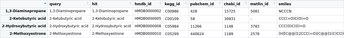
# Parse the response into a table
# Will show mapping to "hmdb_id", "kegg_id", "pubchem_id", "chebi_id", "metlin_id", "smiles"
query_results_text <- content(query_results, "text", encoding = "UTF-8")
query_results_json <- rjson::fromJSON(query_results_text, flatten = TRUE)
query_results_table <- t(rbind.data.frame(query_results_json))
rownames(query_results_table) <- query_results_table[,1]